
library(osmdata)
library(sf)
library(dplyr)
library(ggplot2)
library(ggspatial)
library(rmapshaper)
library(ragg)
library(future)
library(furrr)
library(gifski)I was having lunch at Honest Burgers near campus with a few people and the conversation somehow turned to Byron, the burger chain, and I found myself telling the story of its rise and downfall. Or, at least, a very simplistic version of it based on my limited knowledge of what happened. But that led me to wonder if it would be possible to map the fortunes of Byron. The following is an attempt at doing so.
Finding data
In order to find the data, I use OpenStreetMap data, using the osmdata package in R. The idea is simple: query the Overpass API for restaurants matching our burger chain names within the London bounding box.
My first attempt was to search for restaurants by name:
london <- getbb("London, UK")

if (file.exists("data/london_b.rds")) {
  london_b <- readRDS("data/london_b.rds")
} else {
  london_b <- london |>
    opq(timeout = 120) |>
    add_osm_feature(key = "amenity", value = "restaurant") |>
    add_osm_feature(key = "name",
                    value = c("Byron", "Gourmet Burger Kitchen", "Five Guys",
                              "Honest Burger", "GBK"),
                    match_case = FALSE, value_exact = FALSE) |>
    osmdata_sf()
  saveRDS(london_b, "data/london_b.rds")
}
This highlights some data issues. Of the 3 Byrons in London, this only catches 2. Of the 9 GBK in London, it only catches 3. And I catch none of the Five Guys! You will also notice that I saved the query results to a file, because the API is fairly slow and I do not have the patience to wait for it everytime I update the text of the post (it only times out on a regular basis if you send too many requests in close succession, so this takes care of that too).
Maybe there is some vagueness in the classification and some of these get classified as fast food rather than restaurants? Let’s widen the net:
if (file.exists("data/london_b2.rds")) {
  london_b2 <- readRDS("data/london_b2.rds")
} else {
  london_b2 <- london |>
    opq(timeout = 120) |>
    add_osm_feature(key = "amenity", value = c("restaurant", "fast_food")) |>
    add_osm_feature(key = "name",
                    value = c("Byron", "Gourmet Burger Kitchen", "Five Guys",
                              "Honest Burger", "GBK"),
                    match_case = FALSE, value_exact = FALSE) |>
    osmdata_sf()
  saveRDS(london_b2, "data/london_b2.rds")
}
This is better! I now catch Five Guys, and more of the Gourmet Burger Kitchen (7/9), but still only 2 out of 3 Byrons. Let’s go even wider and include food courts, bars, cafes and pubs:
if (file.exists("data/london_b3.rds")) {
  london_b3 <- readRDS("data/london_b3.rds")
} else {
  london_b3 <- london |>
    opq(timeout = 120) |>
    add_osm_feature(key = "amenity",
                    value = c("restaurant", "fast_food", "food_court",
                              "bar", "cafe", "pub")) |>
    add_osm_feature(key = "name",
                    value = c("Byron", "Gourmet Burger Kitchen", "Five Guys",
                              "Honest Burger", "GBK"),
                    match_case = FALSE, value_exact = FALSE) |>
    osmdata_sf()
  saveRDS(london_b3, "data/london_b3.rds")
}
This doesn’t yield anything further, but it doesn’t hurt to cast the wider net, so I will keep using this query. This is in part because I hope that it makes the query more robust across time periods when amenity classifications may have been different.
I also need to standardize the chain names. The raw name field from OpenStreetMap can vary (e.g., “GBK” vs “Gourmet Burger Kitchen”, or “Byron Burgers” vs “Byron”). A case_when mapping handles this.
Building a reusable query function
Since I’ll need to run this query many times across different dates, let’s wrap it in a function:
query_burger_chains <- function(bbox, datetime = NULL, timeout = 300) {
  q <- bbox |>
    opq(datetime = datetime, timeout = timeout) |>
    add_osm_feature(
      key = "amenity",
      value = c("restaurant", "fast_food", "food_court", "bar", "cafe", "pub")
    ) |>
    add_osm_feature(
      key = "name",
      value = c("Byron", "Gourmet Burger Kitchen", "Five Guys",
                "Honest Burger", "GBK"),
      match_case = FALSE, value_exact = FALSE
    ) |>
    osmdata_sf()

  pts <- q$osm_points[!is.na(q$osm_points$name), ]

  pts |>
    dplyr::mutate(
      chain = dplyr::case_when(
        grepl("five guys", name, ignore.case = TRUE) ~ "Five Guys",
        grepl("gourmet burger kitchen|\\bgbk\\b", name, ignore.case = TRUE) ~ "GBK",
        grepl("honest burger", name, ignore.case = TRUE) ~ "Honest Burgers",
        grepl("byron", name, ignore.case = TRUE) ~ "Byron",
        TRUE ~ NA_character_
      )
    ) |>
    dplyr::filter(!is.na(chain))
}
Going back in time
With OpenStreetMap, it is possible to query the state of the database at any point going back to 12 September 2012, when the licence of the data changed. This is done using the datetime argument in opq().
NoteA caveat
OSM historical data reflects the state of the OSM database at that time. If a restaurant existed but nobody had mapped it yet, it won’t appear. Early snapshots (2012–2014) might have coverage of commercial establishments that is less complete. What we’re mapping is the intersection of “this restaurant existed” and “someone added it to OpenStreetMap”.
I built a series of dates from September 2012 to today, querying roughly every six months, and collected the data using a standalone script that saves each snapshot incrementally. This approach is necessary because the Overpass API can be slow for historical queries and occasionally times out—saving after each successful query means that I only had to run this a bazillion times before having data for all the snapshots.
london_admin <- readRDS("data/london_admin.rds")
london_admin_simple <- ms_simplify(london_admin, keep = 0.15)
all_data <- readRDS("data/all_data.rds")

all_data |> sf::st_drop_geometry() |> count(chain)
chain n
1 Byron 413
2 Five Guys 432
3 GBK 493
4 Honest Burgers 245n_snapshots <- length(unique(all_data$snapshot_date))
date_range <- range(all_data$snapshot_date)
message("Loaded ", nrow(all_data), " records across ", n_snapshots,
" snapshots from ", format(date_range[1], "%b %Y"),
" to ", format(date_range[2], "%b %Y"))Loaded 1583 records across 28 snapshots from Sep 2012 to Feb 2026A first look at the data
Before jumping to maps, let’s look at the count of locations for each chain over time. This gives us a quick overview of what happened:
count_data <- all_data |>
  sf::st_drop_geometry() |>
  dplyr::count(snapshot_date, chain)

ggplot(count_data, aes(x = snapshot_date, y = n, colour = chain)) +
  geom_line(linewidth = 0.8) +
  geom_point(size = 1.5) +
  labs(
    title = "Burger chains in London over time",
    subtitle = "Number of locations in OpenStreetMap",
    x = NULL, y = "Number of locations", colour = "Chain"
  ) +
  theme_minimal()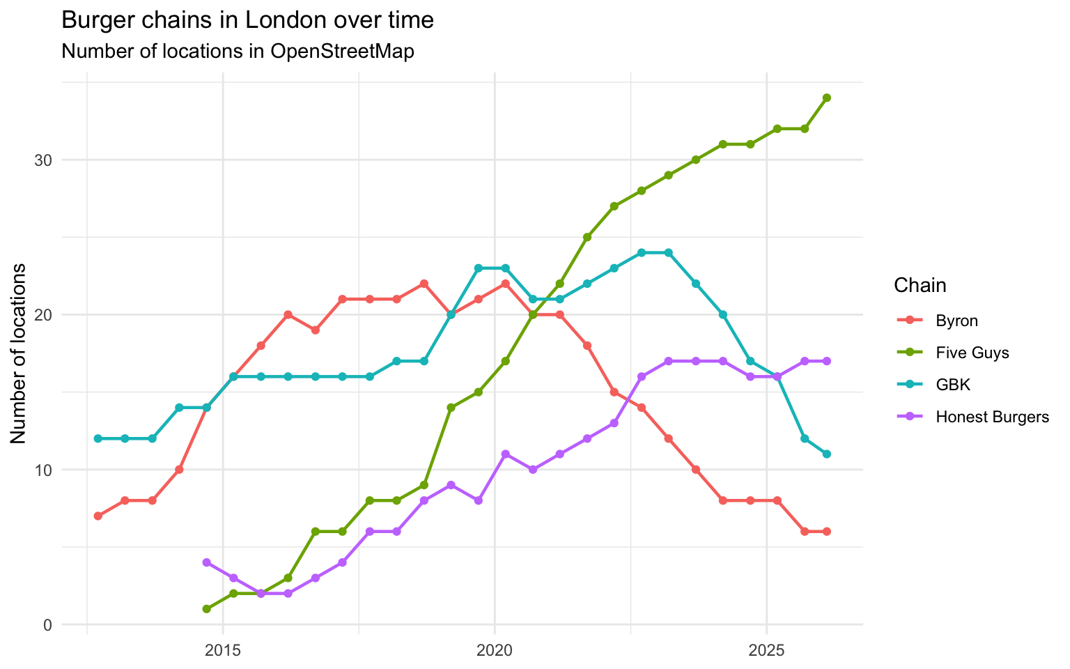
Keeping in mind the OSM data quality caveat from earlier, I suspect that in the first couple of years, the data is likely to underestimates the number of locations.
Mapping the data
Let’s start with a static faceted view, selecting a snapshot roughly every two years to see the broad spatial patterns:
time_points <- sort(unique(all_data$snapshot_date))
selected_dates <- time_points[seq(1, length(time_points), by = 4)]

facet_data <- all_data |>
  dplyr::filter(snapshot_date %in% selected_dates) |>
  dplyr::mutate(date_label = format(snapshot_date, "%b %Y"))

# Order date labels chronologically
facet_data$date_label <- factor(
  facet_data$date_label,
  levels = format(sort(selected_dates), "%b %Y")
)

ggplot() +
  geom_sf(data = london_admin, fill = "grey95", colour = "grey70") +
  geom_sf(data = facet_data, aes(colour = chain), size = 1.5, alpha = 0.7) +
  facet_wrap(~ date_label) +
  labs(
    title = "Burger chains in London",
    colour = "Chain",
    caption = "Source: OpenStreetMap"
  ) +
  theme_void() +
  theme(strip.text = element_text(face = "bold"))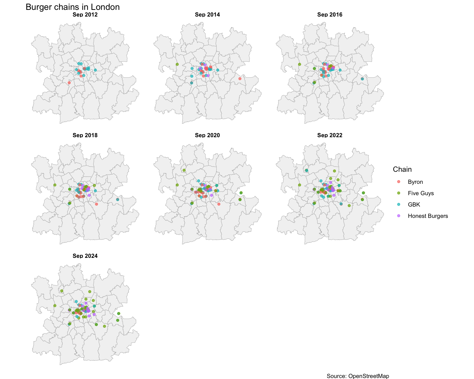
Animating the maps
Now, the thing I really had in mind when starting this was to create an animated map. In order to do that, I render each snapshot as a separate frame using furrr and ragg, then stitch them into a GIF with gifski. Each frame shows the location of the various burger restaurants at that snapshot date.
dir.create("img/frames", showWarnings = FALSE, recursive = TRUE)

unique_dates <- sort(unique(all_data$snapshot_date))

plan(multisession, workers = parallelly::availableCores())

furrr::future_walk(seq_along(unique_dates), function(i) {
  frame_data <- all_data |> dplyr::filter(snapshot_date == unique_dates[i])

  p <- ggplot() +
    geom_sf(data = london_admin_simple, fill = "grey95", colour = "grey70") +
    geom_sf(data = frame_data, aes(colour = chain), size = 2, alpha = 0.7) +
    labs(
      title = "Burger chains in London",
      subtitle = format(unique_dates[i], "%B %Y"),
      colour = "Chain",
      caption = "Source: OpenStreetMap"
    ) +
    theme_void() +
    theme(
      plot.title = element_text(size = 16, face = "bold"),
      plot.subtitle = element_text(size = 12)
    )

  ggsave(
    sprintf("img/frames/frame_%03d.png", i), p,
    width = 8, height = 7, dpi = 200, device = agg_png
  )
}, .options = furrr_options(seed = TRUE))

frame_files <- sort(list.files("img/frames", pattern = "frame_.*png$",
                               full.names = TRUE))
gif_rest <- gifski(frame_files, gif_file = "img/byron_animation.gif",
       width = 1600, height = 1400, delay = 4/3, progress = FALSE)

unlink("img/frames", recursive = TRUE)
Conclusion
The animated map tells a story, though I am not clear exactly which one. Starting this, I had the vision that the map would very clearly show—with more glitter—what the line plot does a pretty good job of illustrating.
Byron’s trajectory is visible: a handful of locations appearing in the mid-2010s, then gradually disappearing as the chain contracted. Meanwhile, Five Guys and Honest Burgers have been steadily expanding, filling the gaps that Byron and others left behind.
But all of this you can already get from the line plot. The one thing that I think is visible on the map but not in the line plot is that for a lot of the restaurants location, it seems that they tend to appear close to where there is already another burger place. Now, there is probably a better way to bring this out of the data, but I need to think more about how to do that.
Overall, I am impressed by what one can do using OpenStreetMap data with osmdata, sf, and ggplot2 in R.
Citation
BibTeX citation:
@online{vernet2026,
  author = {Vernet, Antoine},
  title = {The Rise and Fall of {Byron,} in Maps},
  date = {2026-04-02},
  url = {https://www.antoinevernet.com/blog/2026/04/byron/},
  doi = {10.59350/hjr0m-03b71},
  langid = {en}
}
For attribution, please cite this work as:
Vernet, A. 2026, April 2. The rise and fall of Byron, in
maps. https://doi.org/10.59350/hjr0m-03b71.